Solving the Pricing Riddle with Machine Learning
Can you solve this Christmas tree price elasticity riddle?:

We pose this pricing challenge to highlight an inherent difficulty in working with price elasticities to optimize prices.
The assumption is that the price elasticity contains all the relevant information a pricing manager needs to know about how demand reacts to a price change. This is implicit in all elasticity-based price solutions.
Why are price elasticity pricing solutions problematic?
Consider the two most widely used demand functions: linear and exponential demand.
Under linear demand, absolute volume changes are proportional to absolute price changes. For example, for each €5 price increase, you lose 10 sales units.
Under exponential demand, relative volume changes per relative price change remain constant. For example, you lose 10% in volume for every 5% price increase.
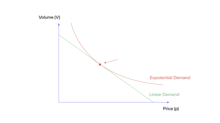
Figure 1 shows these two demand functions. Pricing on elasticity only works if differences between demand functions and their implications for volume changes are also minor and can be neglected—at least for smaller price changes. If the choice of demand function has real implications, then pricing on elasticity can become dangerously misleading.
So, let’s investigate how to react to a cost increase under linear and exponential demand, using Tim’s case as an example.
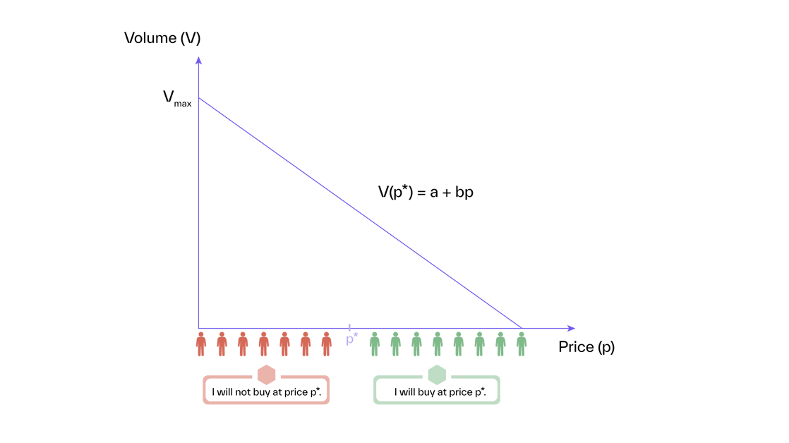
Linear demand
Under linear demand, the relation between volume (V) and price (p) is:
...where a is the maximum volume if the product is ‘sold’ at price 0, and b is the slope of the demand function. If sales drop with increasing price, then b is negative. This is the normal case.
Figure 2 shows the linear demand function and its underlying assumption about customers’ willingness to pay: If customers were lined up, with each customer “standing” on their willingness to pay, the distance between customers would remain the same.
In other words, you lose the same number of customers if you increase from €10 to €20 or from €70 to €80.
Then, price elasticity (ε) is:

 ...where c is cost.
How should Tim react to the €5 cost increase from €50 to €55 in the Christmas tree example so that he is again in the profit optimum?
Following the linear demand equation, half of the absolute cost increase should be passed on as a price increase. That means that the price of the tree needs to be increased by €2.5 to €102.5. As a result, Tim loses 5% of his sales volume, 3% of his revenue, and 10% of his profit. This is the best he can do under linear demand.
Exponential demand
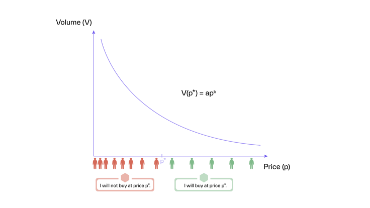
Under exponential demand, volume (V) is defined as a function of price (p):
 ...where a is a constant, and b is the price elasticity. If sales volumes decrease with price increases, then b is negative. This is the normal case.
Figure 3 shows the exponential demand function and its underlying assumption about customers’ willingness to pay: As prices decrease, the distribution of customers densifies constantly.
The price optimum is then at:
 ...where c is cost.
How should Tim react to the cost increase in the Christmas tree example so that he is again in the profit optimum?
Following the exponential demand equation, the percentage cost change must change the price. That means that if the cost of a Christmas tree increases by 10% (or €5), then the price of the tree also needs to increase by 10% (from €10 to €110). As a result, Tim loses 17% of his sales volume, 9% of his revenue, and 9% of his profit. This is the best he can do under exponential demand.
Conclusion
It is important to note that Tim will always lose money with elastic demand if he is at the optimum before the cost increases. However, his price change differs greatly depending on the assumed demand function.
Under linear demand, he passes on half of the absolute price change. In contrast, under exponential demand, he passes on twice the absolute price change to keep his margin constant and stay within the optimum profit.
That is quite a meaningful qualitative difference, and in our example, a significant actual difference of €110 – €102.5 = €7.5.
Linear and exponential demand are extreme cases and can be considered reasonable boundaries of Tim’s actual demand. Imagine a consultant who has correctly measured Tim’s price elasticity of -2 but cannot be sure about the underlying type of demand function. For them, the honest recommendation to Tim is that he should increase his price by something between €2.5 and €10. If Tim is like most vendors, he would probably have gone for a €5 increase on his own.
In summary, if vendors already price at or near the price optimum, pure elasticity-based pricing adds very little in scenarios such as the Christmas tree case. It might actually be harmful if it ignores behavioral considerations.
Get Started Today to Reach Your Goals Tomorrow
Buynomics' pricing solution, which uses Virtual Shopper AI to predict demand reactions to price changes, addresses the shortcomings of pricing on elasticity.
Request a demo today to see how Buynomics supports your Revenue Growth Management team and helps you make data-driven pricing decisions.