Price Elasticity - the Good, the Bad and the Ugly

Price is the most important profit lever. Being able to increase price without a loss in demand is more profitable than increasing units or decreasing variable or fixed costs. Unfortunately, demand reacts to price changes, and a price increase – in general – leads to a decrease in demand. Therefore, measuring how customers react to price changes is crucial. This is done using the price elasticity of demand – in short: price elasticity.

In this, and two follow-up blogs, we take a closer look at key facets of price elasticity: 

The Good: How in simple cases, price elasticity can be used to maximize revenue or profit. 
The Bad: How in most cases, price elasticity cannot be estimated with the necessary precision to be useful for pricing. 
And the Ugly: How pricing on price elasticity completely falls apart in a market with multiple products and competition.

Price elasticity describes the relationship between price and demand. It is defined as the ratio between the percentage change in demand and the percentage change in price*. For example, if the price is increased by 1% and consequently demand decreases by 2%, the price elasticity is -2% / 1% = -2.

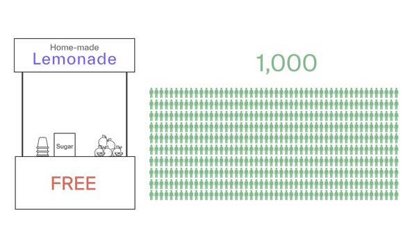
Let’s see if we can bring these equations to life using a simple example. Assume we operate a lemonade stand and we want to find the ideal price. We offer only one product, a cup of lemonade, and we are the only supplier in town.

We have costs of $0.50 per cup (for lemons, sugar, ice, water and the cup) and from a “Free Trial”, we know the market size is 1,000 cups per day.

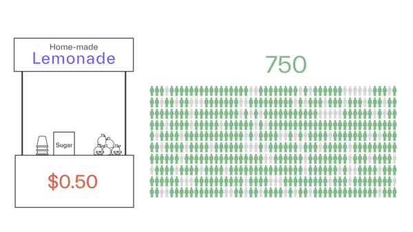
If we charge $0.50 per cup (i.e. zero margin), we sell 750 cups. This means that 250 people have a willingness to pay of less than $0.50. We make a revenue of 750 * $0.50 = $375 and a profit of 750 * ($0.50 – $0.50) = $0.

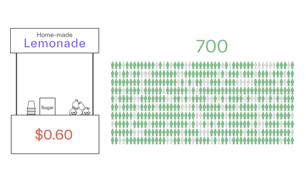
If we increase the price to $0.60 (+20%), we lose another 50 people, who have a willingness to pay between $0.50 and $0.60, and sell 700 cups (-6.7%). Therefore, the price elasticity for this price range is -6.7% / 20% = -0.33. Our revenue is 700 * $0.60 = $420 and our profit is 700 * ($0.60 - $0.50) = $70.

If we continue this experiment by changing the price in steps of 5 cents until no one buys from us anymore, we get the relationship between price and demand shown in Graph A.

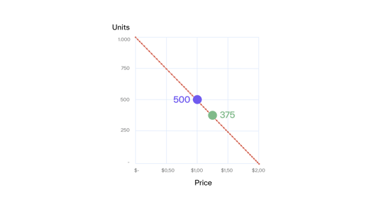
Graph A

Our price demand function is linear, i.e. we lose the same absolute number of units for every 5 cents we increase the price. In this example, demand is determined only by our price. In realistic situations demand is influenced by more factors. The most important are:

• Seasonality, events (the weather, holidays, etc.), and chance (if individual people feel like having lemonade today). We will look at the influence of this in the next blog.
  
  
• Alternative options from ourselves (if we also offer grapefruit juice at a certain price) and competition (a lemonade stand across the street). We will look at this in blog 3 of this series.

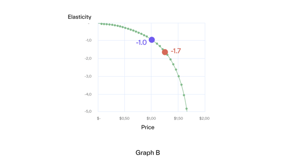
Inelastic price range

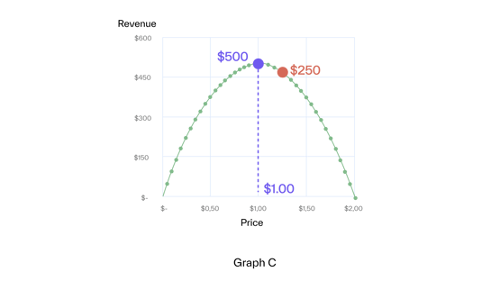
The price range with an (absolute) elasticity of less than one (in our example from $0.00 to $1.00) is called inelastic. In the inelastic range, we gain revenue by increasing price (Graph C), since the percentage decrease in demand is smaller than the percentage increase in price. The maximum revenue is reached at the limit of the inelastic range, at elasticity -1, where marginal units loss equals marginal price increase. This rule applies in general.

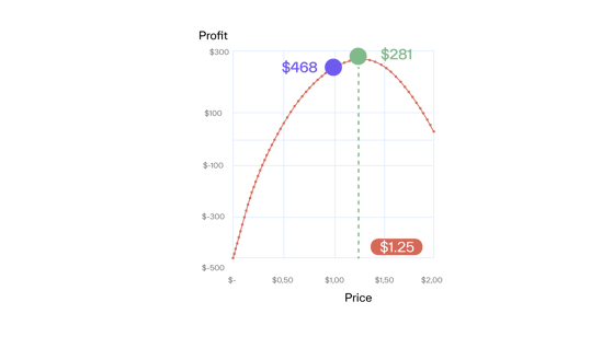
Because profit is always smaller than revenue (for non-zero costs), profit also increases (Graph D). Therefore, in the inelastic range, price increases are a good idea regardless of whether you care for revenue or profit.

Elastic price range

The price range with an (absolute) elasticity of more than one (in our example above $1.00) is called elastic. Here, the percentage decrease in volume is larger than the percentage increase in price, i.e. we lose revenue when we increase price. However, profit keeps increasing with price to the point where Margin * Elasticity = -1. In our example, this is the case for a price of $1.25 (Graph D).

We see from that formula that, the lower the margin, the higher the elasticity at the profit optimum – and consequently, the larger the difference between the revenue and profit optimal price. For example, if there was a bad harvest, lemon prices explode and our costs double to $1.00 per cup, we need to move much further into the elastic range, to $1.50, to optimize our profit. Here the margin is 33% and the elasticity is -3. We passed half of our cost increase (+$0.50) on to customers as a price increase (+$0.25). This is a general rule for linear demand functions: If cost changes, half of the change should be passed on to customers to stay at the profit optimum. For other demand functions, costs are passed on differently. For example, in the case of the multiplicative demand function, the percentage price change must be equal to the percentage cost change – i.e. in the example above with a cost increase of 100%, the price increase would also have to be +100%, which leads to a new price of $2.00 vs. the $1.50 under a linear demand function. Pricing is very sensitive to understanding demand!

Conclusion

The Good about price elasticity is, we can use it to determine the optimal prices for revenue and profit***:

• In the revenue optimum: Elasticity = -1

• In the profit optimum: Elasticity * Margin = -1

In the next blog we will investigate the Bad (measurement) and the Ugly (multiple products and competition) of price elasticity.

:
* Precise definition: Ε = ∂Q/Q / ∂P/P.

** In the literature, a multiplicative price demand functions Q = α ∗ Pβ (Q: demand; α: constant; P: price; β: elasticity) is commonly used. It is the only demand function with constant elasticity (Ε = ∂Q/Q / ∂P/P = ∂Q/∂P ∗ P/Q = β ∗ α ∗ P(β-1) ∗ P/Q = β ∗ Q/Q = β). We will have a closer look at it in the next blog.

*** This optimizes the price for one product. With several products, the prices that optimize total revenue or profit differ from the prices that optimize each product individually (blog 3 in this series).