
The Truth About Price Elasticity
"Price elasticities are like sausages; everyone likes them, but it’s better not to see them being made."
Understanding the customer is the most important aspect of pricing, and measuring price elasticity is a widely used method for doing so.
More specifically, price elasticity is measured to answer the question: “How have customers adapted their purchasing behavior to price changes in the past?” From this, it can be deduced how to set prices in the future to achieve pricing goals (e.g., optimize profit, revenue, or market share).
In our last article on price elasticity, we discussed the general concept and saw how to set prices to maximize profit or revenue, given a precisely measured price elasticity.
In this blog, we will focus on measuring price elasticity itself and the reliability of results.
Recap—How Does Price Elasticity Work?
We operate the only lemonade stand in town and offer exactly one product: lemonade.
We tested prices from $0.00, where we “sold” 1,000 units per month, to $2.00, where no one bought from us anymore (Graph A). The corresponding elasticity is shown in Graph B.
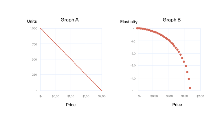
Note that the elasticity is not constant but changes with price. Although this is true in reality, we need to assume a constant elasticity over a limited price range to determine it by linear regression*.
In the initial scenario, we made two more assumptions that are oversimplified and need to be adjusted:
- We tested the full price range (from $0.00 to $2.00) in increments of $0.05. However, this will not be possible unless the revenue growth manager works for a very relaxed CEO / CFO. Rather, if you have an experimental mindset, you will test prices in a much narrower range (e.g., +/- 10%). Often, prices are not intentionally “tested” but come from more or less thought-out rules.
- Most importantly, there is zero noise in the data. In other words, price is the only factor that influences the purchasing decision—not weather, vacations, concerts, football games, or pure chance. Of course, that’s not realistic.
Let’s assume that we have operated our lemonade stand for one year and didn’t really care much about pricing. We simply used a cost-plus pricing strategy and calculated our price by doubling the cost to get a 50% margin.
We adapted our prices approximately every other week to changing costs. We plot our 48 price/unit combinations to determine the price elasticity and fit the demand function on the data**. The result is shown in Graph C.
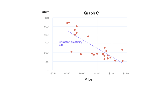 The units no longer lie on a straight line as in Graph A’s ideal world.
Of course, there are other influences on buying behavior than price. These other factors show up in Graph C as “noise.” This noise can be attributed to two main sources: systematic and random noise.
Systematic noise
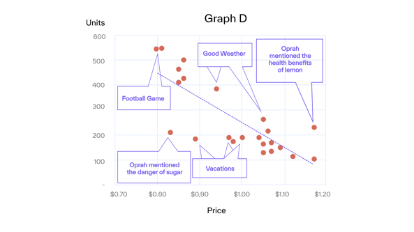
External circumstances can, in principle, explain systematic noise. For our lemonade stand, we thought hard and came up with the explanations in Graph D.
All influencing factors could be considered extensions to the price-demand function. In reality, this may work for more obvious and reliable factors, such as seasonality or vacations. In contrast, many sources (like a private party) will be unknown, and/or the corresponding data will not be available or trustworthy.
Even if all data were available, we still need to translate an influencing factor (e.g., temperature) into the proper mathematical term. We also need to consider the interconnection of different influencing factors.
For example, how would you consider these interconnected factors:
- August (higher consumption)
- during the first two weeks of vacation time (lower consumption),
- with higher than normal temperature (higher consumption),
- but a lot of rain (lower consumption),
- that has mainly fallen at night (higher consumption)?
When in doubt, it is better to exclude sources. Otherwise, the model will be overfitted, leading to substantially worse results than excluding potential sources in the first place.
John von Neumann once said, “With four parameters, I can fit an elephant, and with five, I can make him wiggle his trunk.”
Random noise
Random noise arises from stochastic fluctuations and cannot be predicted. For example, the number of potential buyers who feel like having lemonade today (before they even consider prices) is a source of random noise.
No way to eliminate or correct pricing for random noise exists except by increasing the sample size.
The "Bad" in Price Elasticity
Since we have now considered all the noise, we want to know how reliable this result is before we change our prices. In other words, how much noise is acceptable for valuable price decisions? Unfortunately, the answer is not much.
Table E shows the level of noise and the corresponding reliability of elasticity and derived prices***.

Let’s look at the example of “10% Noise” to understand better what is happening here.
The 10% noise means that 10% of the variation in demand cannot be explained by price. This is actually very little. If we sell 100 units on average per month, this corresponds to an unexplainable deviation of 10 units. This could be caused by a BBQ in the neighborhood (+10) or a regular customer’s vacation (-10).
The 10% and 25% noise graphs look very smooth for everyone who has ever determined elasticities with real data. Even the 50% noise graph looks much cleaner than most data seen in real life.
But even 10% noise leads to considerable uncertainty in elasticity. From 10,000 simulations, 95% of determined elasticities are within -2.5 and -1.5 (where the true elasticity is -2). If we determine the optimum price based on these elasticities, our average error is 11%. For 25% noise, the error is 36%.
In other words, if the ideal price is $1.00, the price determined from elasticity measurement is, on average, as bad as $1.36 (or $0.64). This is hardly acceptable.
Understanding the customer is at the core of good pricing. Leveraging sales data is often the only way to do this, and, as we now see, elasticity is a poor approach.
Get Started Today to Reach Your Goals Tomorrow
Request a demo today to see how Buynomics supports your RGM team and helps you make data-driven decisions across all RGM levers, including pricing.
* The only price demand function—our hypothesis of the true relationship between price and demand—with constant elasticity is:
Q = α ∗ P^β (Q: demand; α: constant; P: price; β: elasticity).
It has constant elasticity (e.g., the elasticity does not depend on price) since
Εlastictiy = ∂Q/Q / ∂P/P = ∂Q/∂P ∗ P/Q = β ∗ α ∗ P^(β-1) ∗ P/Q = β ∗ Q/Q = β.
To determine price elasticity, the function is logarithmized
log(Q) = log(α) + log(P) * β.
If we plot log(Q) over log(P), we get the elasticity β as the slope.
** Actually, we do a linear fit on the logarithms of price and demand (see *).
*** To generate the test dataset, 24 periods have been simulated. Each period has one price and corresponding demand. The price for every period was randomly drawn between $0.90 and $1.10. The corresponding “Ideal World” demand has been calculated according to the price demand function Q = α ∗ P^β (with alpha = 500 and true elasticity β = -2). Two random numbers have been added to these “Ideal world” sales to simulate noise.
1. Random noise, drawn from a binomial distribution, which cannot be controlled for.
2. Systematic noise of X% by multiplication of the “Ideal World” sales with a random number between 1-X and 1+X (e.g., 10% noise by multiplication of a random number between 0.9 and 1.1). The logarithmized price demand function was fitted on this dataset to estimate the elasticity β.

.png?width=520&height=294&name=The%20Revenue%20Manager%20of%20Tomorrow%20(1).png)
